Extracting important information from medical documents using Named Entity Recognition with Bidirectional LSTM and Convolutional neural networks

2.1 Introduction

Growth in Artificial intelligence (AI) in Medical domain has been drastic, natural language processing, image processing and computer vision are few of the main topics in which the medical domain has been helped a lot. Natural Language Processing (NLP) has been widely active in research area for medical informatics. NLP services have the potential to connect relevant insights from data that was provided in text form. NLP in healthcare media can accurately give voice to the unstructured data of the healthcare universe. Named-entity recognition (NER) (also known as (named) entity identification, entity chunking, and entity extraction) is a subtask of information extraction that seeks to locate and classify named entities mentioned in unstructured text into pre-defined categories such as person names, organizations, locations, medical codes, time expressions, quantities, monetary values, percentages, etc. As NER is the first step in the text processing, where the entities are extracted from the unstructured data (medical – electronic health record systems). The entities extracted from the unstructured data can be medicines, diseases, treatments, symptoms, patient’s name, and histology information’s.

2.2 Data set description

In this study, annotated corpora from the 2014 SemEval competition and the 2010 i2b2 challenge were utilized. The problem, test, and treatment are three different categories of clinical entities that are annotated in the i2b2 2010 corpus. In total, 268 annotated discharge summaries from the i2b2 challenge were used in this work (17 from the training set and 251 from the test set). There are 27,589 entities, 326,474 words, and 9,689 sentences in this annotated corpus. Every entity is made up of a series of words. Only one sort of entity, the disorder mention, is present in the SemEval corpus. However, the SemEval corpus includes disconnected entities, or entities made up of many text regions. The medical notes of SemEval 2014 are made up of Disorders, Discharge notes, ECG and ECHO readings of patients. Training set has Notes around 300 and Entities of 11,156 in it, testing includes 133 Notes and 7971 Entities.

2.3 Data pre-processing

A BIO format was created out of the annotated corpus of i2b2. It specifically classified each word into one of the following classes: B denotes the start of an entity, I denote its interior, and O denotes its exterior. We have six different B classes and six different I classes because there are six different entity kinds. For instance, we define the B class as “B-m” and the I class as “I-m” for drug names. Consequently, each word has a total of 13 different classes (including O class). This changes the whole dataset into a multi class classification problem. Stop words are used to remove words that are common and doesn’t denote any medical terms. Tokenization is used after removing stop words, as it is a technique used in natural language processing to break down phrases and paragraphs into simpler language-assignable elements. The collecting of data (a sentence) and its breakdown into comprehensible components are the first steps of the NLP process (words). After tokenization, we perform lemmatization process to the tokens present in the dataset. Lemmatization is the process of grouping words with the same root, or lemma, but various meaning derivatives or inflections, so they can be studied as a single unit. To reveal the word’s dictionary form, inflectional suffixes and prefixes are to be removed.

2.4 Text processing

After tokenization and lemmatization, we will be creating indices dictionary for both word (Tokens) and tags (class labels). These indices are used when performing operations to join both word and tags to form a single token for training and testing the data while modeling. We then change greek letters to ascii characters for the machine learning models to understand the given text. There are two main text processing layers that is followed in this study to perform before modeling, they are padding sequence layer and embedding layer.

The same form and size of inputs are necessary for all neural networks. The sentences do not all have the same length, though, when we pre-process and use the texts as inputs for our model, such as LSTM. To put it another way, it makes sense that some of the sentences are longer than others. The padding is required since we must have inputs of the same size. Additionally, we may provide a maximum word count for each sentence, and if a sentence goes above that limit, we can exclude some words. This process is known as padding sequence, this process has two types, post and pre truncation. ‘Post’ padding adds zeros to the starting of the sentence and ‘post’ adds zeros to the end of the sentence.

After performing padding, we then use embedding layer where we can turn each word into a fixed-length vector with a predetermined size. The resulting vector is dense and does not only contain 0s and 1s, but also real values. Word vectors’ fixed length and decreased dimensions enable us to express words more effectively. The embedding layer functions thus way like a lookup table. In this table, the dense word vectors serve as the values and the words serve as the keys.

2.5 Word embedding and character level embedding

With word embedding, words are translated into low-dimensional vectors in a distributed manner. Utilizing a word vector has the benefit of capturing a word’s meaning or relationships to other words. We use pre-trained word vectors from major biomedical corpora that are openly accessible in our model. Pre-trained word vectors developed using biomedical corpora are useful for capturing each entity’s biological meaning because some words in the biomedical literature are not frequently used. Character-level embedding is also used to represent input tokens in addition to word embedding. When OOV words are encountered that are not present in the learned word vectors, this technique is applied. Character-level embedding is helpful for efficiently extracting the morphological information of each word token, especially in the biomedical domain where multiple unique words exist in irregular forms. To extract the character-level information, we employ the CNN and bi-LSTM neural networks, two separate neural networks.

2.6 Model Building

For this study we will be building the model using Bi-LSTM and 1D- CNN, For handling the 1-dimensional data, 1D-CNN uses 1-dimensional convolution layers, pooling layers, dropout layers, and activation functions. The following hyper-parameters are used to configure 1D-CNN: the number of CNN layers, the number of neurons in each layer, the size of the filter, and the subsampling factor of each layer. The filter is initially applied to an input through the convolution layer. A feature map, which shows the specific qualities associated to the data points, is created by repeatedly using the filtering procedure. A set of weights were used to contain the multiplication of inputs during the linear convolution process. In this instance, the single-dimensional array weights, or kernel, are multiplied by the inputs (Qazi et al., 2022). The per-character feature vectors, such as character embedding’s and character type, are used to extract a new feature vector for each word using convolution and a max layer. Depending on the CNN window size, PADDING characters are appended to the ends of words to pad them. CNNs, which were first utilized in image processing, are now frequently employed in a variety of NLP tasks. We use CNN to efficiently extract local information from each input token’s characters. A character vector is assigned to each character in the word token. Then, the filters of various sizes are applied to the embedding matrix to extract significant characteristics of nearby inputs. In the convolution process, we employ three distinct filter widths to capture diverse information. A max-pooling technique is used in CNN’s last step to extract a single feature from each of the feature maps. The local information is preserved by concatenating the output characteristics to represent each word.

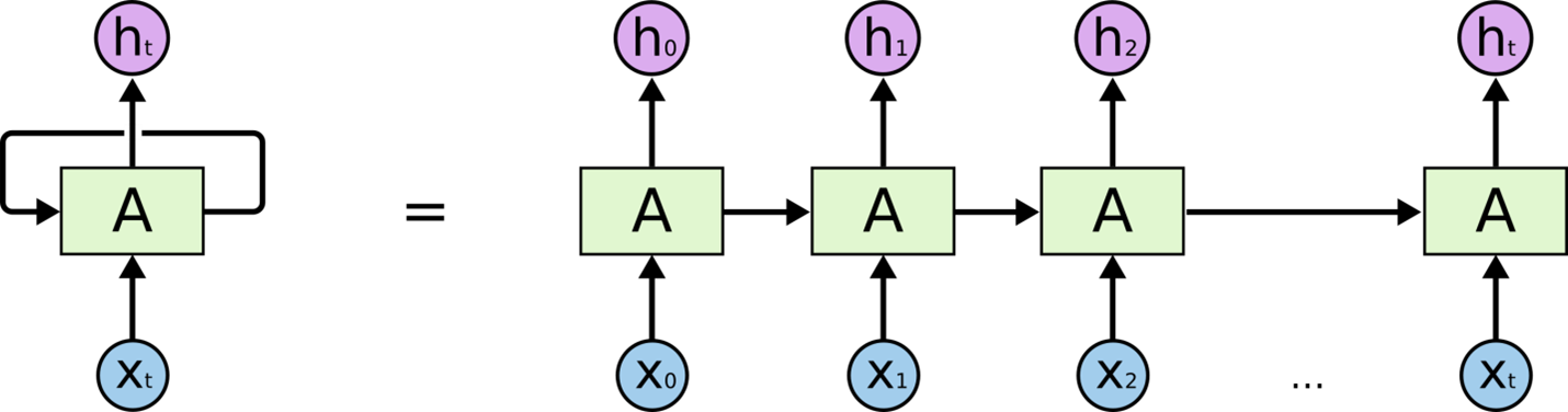
Then to perform modeling on Bi-LSTM after CNN, we need to construct as simple recurrent neural network algorithm for better understanding. A recurrent neural network (RNN) is a class of artificial neural networks where connections between nodes form a directed or undirected graph along a temporal sequence. This allows it to exhibit temporal dynamic behavior. Derived from feed forward neural networks, RNNs can use their internal state (memory) to process variable length sequences of inputs (Wikipedia, 2022). Below is the image of simple recurrent neural network rolled out.

The term “long short-term memory” (LSTM) refers to recurrent neural networks that have multilayer cell structures, state memories, and state memory. LSTMs were built expressly to get around recurrent neural networks’ problem with long-term dependence. Although the repeating module of LSTMs also has a form akin to a chain, it is different. There are four neural network layers, interacting in a highly unique way, as opposed to just one. In that they offer a comparatively straightforward solution to the vanishing gradient problem, LSTM-based models outperform RNNs. The LSTM models, which function as a kind of extended memory for the RNNs, enable them to learn and remember long-term dependencies of inputs. Three gates make up the LSTM model: forget, input, and output gates. The input gate defines how much new information will be added to the memory, the output gate determines if the value already present in the cell contributes to the output, and the forget gate determines whether to maintain or discard any existing information. The choice is made by a sigmoid layer called the forget gate. It accepts input at ht-1 and xt for each number in the cell state Ct-1 and outputs a number between 0 and 1 for each number in the range.

Architecture of LSTM is given below,

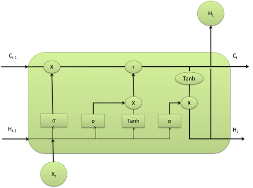
A 1 indicates that the material should be saved, but a 0 indicates that it should be deleted. Which values should be updated next is decided by the input gate layer, which is the following sigmoid layer. A Tanh layer then generates a vector of fresh candidate values, C’t, and updates the state with these values. In the following phase, these two will be blended to create an updated state.

All of the tokens are transformed into their embedding vectors during the word embedding step. Lemmas are additionally transformed into their WE vectors and joined to the preceding vectors. PoS tags, orthographic and morphological traits, such as digit/non-digit, initial character uppercase, and all characters uppercase, were also introduced. The embedding vectors are then added to a BiLSTM layer that has a foTo convert word characteristics into nrward layer and a backward layer. Since the former analyses data from left to right, it allows the network to store information from the past to the future. The network can perform the opposite of the backward thanks to the forward layer. The values of the cell state are then sent to the sigmoid layer, which decides which parts of the cell state we’re going to output. We pass the cell state through Tanh and multiply it by the output of the sigmoid gate to only output the significant portions after pushing the values to be between 1 and 1. Additionally, character-level characteristics are extracted using bidirectional LSTM models. To create a fixed-size vector that represents a word token, we apply the bi-LSTM across the sequence of character embedding for each word and concatenate the two final hidden states from the front and backward LSTM. The model can keep both past and future knowledge by utilising bidirectional hidden states. The bi-LSTM model also well captures the general characteristics of each word token.

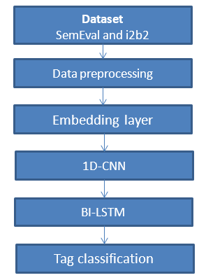
To convert word characteristics into named entity tag scores, we used a stacked bi-directional recurrent neural network with long short-term memory units. Each word’s retrieved features are sent into a forward and a backward LSTM network. A linear layer and a log-softmax layer decode the output of each network at each time step into log-probabilities for each tag category. To create the final product, these two vectors are simply joined together. Below is the framework of the methodology,

In order to allow the network to take into account the neighbor tags, the output of the BiLSTM layer is finally incorporated into the CNN layer. In other words, it enables the network to establish tag relationships. For instance, if a token is associated with the start of a named entity, the token that follows it is likely the continuation of that named entity. This layer is also in charge of preventing the in-named entity tag from being applied to a token without the named entity first being begun. A learning rate of 0.001 was employed with the Adam optimization algorithm. Since the application of these models to English is the main focus of this study rather than the architecture, a grid search was not conducted. We used 50 training epochs and 10-fold cross validation to conduct a grid search to determine the optimal number of hidden units and dropout rates for our model. We only utilized a restricted variety of options for the grid search of the number of concealed units 23 due to the dataset’s sparse instance count.

2.7 Model architecture

To build a model with input as words we need to create an embedding layer with input dimension as number of words and output dimension as the maximum length considered in the data processing step. So as discussed above we will have 180 dimension data as the embedded matrix which will be the input to the model.
Then we pass the outputs of Embedding layer to 1D CNN model that we have created to perform feature extraction technique.
We then add Bidirectional long short term memory cells. We also should set the return sequences as true in this layer to pass on the hidden state results to the next layer.
The bi-LSTM has two layers with forward LSTM and Backward LSTM stacked after the 1D-CNN layers. Then we add a single dense layer to connect all the output cells of the backward LSTM.
Then we add another dropout layer and add activation as the softmax function, we also set the optimizer as “ADAM” and set loss as “categorical cross entropy”. We then set the batch size as 1280 (multiples of *128).

ALGORITHM – 1D-CNN + BI-LSTM

INPUT – Medical notes and patient information

OUTPUT – Important keywords with tags classification

BEGIN –

Function – preprocessing:

Stop words removal
Lemmatization
Greek words to ASCII characters

Function – padding and train, test split:

Padding sequencing is applied on the preprocessed data.
Split the data set into training and test dataset for training the model. The data is split into 70% and 30% for training and testing set respectively.

Function – Modeling:

X <- training and testing dataset (cleaned dataset with social media posts)
Embedding layer <- X
CNN features output <- CNN CELLS (Embedding layer output)
BI-LSTM output <- BI-LSTM CELL (CNN features output)
Tag scores <- Dense layer (BI-LSTM output)
Target class <- MAX (Tag score)

Function – Prediction:

Check for the training and testing scores using Accuracy, f1score, precision and recall.
To achieve better accuracy hyper parameter tuning is performed for variables such as batch_size, filter, nodes, embedding dimension, learning rate and optimizer.
To predict new data, run the preprocessing function on it and run the trained model.

END

2.8 Result

2.8.1 Model training

From the model explained in methodology, we then train the dataset on it for 7 epochs to achieve better accuracy. We can see the training stage of our model below,

2.8.2 Hyper-parameter Optimization

Based on the performance of the development set, we ran two rounds of hyper-parameter optimization and chose the optimal settings. Following the use of several optimization approaches, the final hyper-parameters are displayed in the table below.

Hyper parameters	I2B2 dataset	SemEval
LSTM Layer	2	5
CNN Layer	2	1
LSTM Cell	100	150
CNN filter size	3 * 3	5 * 5
CNN No. of filters	32	16
Learning rate	0.001	0.0001
Epochs	10	15
Dropout	0.30	0.40
Batch size	32	64
Padding	Yes	Yes
CNN output size	32	64

In the first round, we used random search to choose the optimal hyper-parameters from the i2b2 data development set. About 500 hyper-parameter settings were examined. The learning rate and epochs were then adjusted using the identical settings on the validation set for both datasets. Using Optunity’s particle swarm implementation, we conducted independent hyper-parameter searches on each dataset for the second round because there is some evidence that it is more effective than random search. This time around, we also assessed 500 hyper-parameter options.

2.8.3 Word embeddings

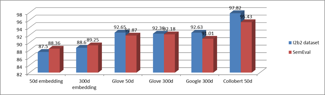
The table below demonstrates that, independent of the additional features applied, we gain a big, significant improvement when trained word embeddings are employed as opposed to random embeddings. The performance of various word embeddings in our top model (BLSTM-CNN + embedding) is also contrasted in the table below. The publicly accessible GloVe and Google embeddings for i2b2 lag behind random embeddings by around one point. Additionally, there is little to no difference between 50 and 300 dimensional embeddings –

Embeddings	I2b2 dataset	SemEval
50d embedding	87.5	88.36
300d embedding	88.6	89.25
Glove 50d	92.65	91.87
Glove 300d	92.36	92.18
Google 300d	92.63	91.01
Collobert 50d	97.82	95.43

One potential explanation for why Collobert embeddings outperform other publicly accessible embeddings on I2B2 is that they were trained on a vocabulary that is best suited for named entity recognition because it contains all of the accepted medical terms, as opposed to the other embeddings, which were not. In instance, Google’s embeddings were trained case-sensitively, and embeddings for numerous popular punctuation marks and symbols were not provided. As a result, we suspect that Google’s embeddings perform poorly due to vocabulary mismatch. We conducted experiments utilizing new word embeddings that had been trained using GloVe and word2vec, along with a vocabulary set, to test these predictions. Our word2vec skip-gram embeddings outperformed Google’s embeddings on Sem EVal, while our GloVe embeddings outperformed publically available embeddings on CoNLL-2003. Optimizing them all will probably produce better results and provide a more accurate comparison of word embedding quality because word embedding quality depends on the hyper-parameter choice made during their training and because in our NER neural network, hyper-parameter choice is probably sensitive to the type of word embeddings used.

2.8.4 Datasets

Dataset	Training accuracy	Testing Accuracy
SemEval	97.72	96.25
I2B2	95.43	94.62

2.8.5 Performance metric

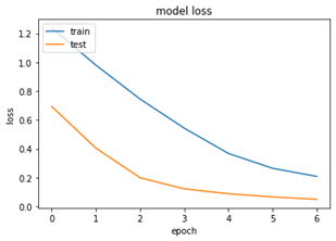
We have achieved an accuracy of 95% with limited amount of epochs and convolutional neural network and bi- directional long short memory. We can see the below accuracy and loss graphs for the trained model –

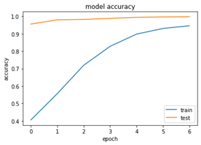
The model accuracy graph shows us the training set and testing set have gradually increased until the end of epochs and the gap between them decreases drastically. Same goes for the loss model below.

Validation accuracy has been boosted to 97.72 accuracy at the end of the 7^th epoch; this is higher than the training accuracy. This might because we might have had set of classes which are in training set which the model has learned well and most of the testing set would have go that particular class in it. Shuffling the data set might give us some information on this situation.

2.8.6 Effects of character level embedding

We ran experiments using models with four distinct embedding combinations to examine the effects of various character embeddings and the impact of the fully connected network that is used to merge character and word vectors. The table below shows the findings. In experiment 1, the model solely employed the word-level embedding (WE), while in experiments 3 and 5, the models combined the word-level embedding with a particular kind of character-level embedding (CNN or bi-LSTM). Character-level embedding is helpful for handling OOV words in NER tasks, as shown by the results of experiments 3 and 5, which greatly surpassed those of experiment 1. Additionally, in tests 3 and 5, the bi-LSTM model outperformed the CNN model in extracting character-level features for the i2b2 dataset while the opposite was true for the SemEval dataset. This suggests that the CNN and bi-LSTM models produce equal results when extracting character-level characteristics. 7th experiment, we looked examined the impact of combining the word-level embedding with two different character-level embeddings. The suggested model, which uses all three types of embedding for word representation (char-bi-lstm, char-cnn, and word), performed best for both datasets in tests 3, 5, and 7, reaching accuracy of 97% and 95% for the abovementioned datasets.

2.8.7 Effect of Dropout

To isolate the impact of dropout on both the validation set and testing data sets, the models for each dataset are trained using only the training set. All other hyper-parameters and features remain the same as our best model. Dropout is crucial for cutting-edge performance in both datasets, on both the validation set and the testing data sets, and the improvement is statistically significant. Based on the validation data set, dropout is optimized. When considering drop out values as 0.1, 0.2, 0.3, 0.4 and 0.5, 30% of drop out worked better in both the dataset. When 0.3 is fixed as drop out value 97% in i2b2 and 95% in SemEval.

Drop out	I2B2 dataset	SemEval
0.1	88.6	88.36
0.2	92.65	89.25
0.5	92.36	91.87
0.4	92.63	91.01
0.3	97.82	92.18

2.9 Conclusion

We have shown that our neural network model, which incorporates a bidirectional LSTM and a character-level CNN and which benefits from robust training through dropout, achieves state-of-the-art results in named entity recognition with little feature engineering. Our model improves over previous best reported results on two major datasets for NER, suggesting that the model is capable of learning complex relationships from large amounts of data. Preliminary evaluation of our partial matching lexicon algorithm suggests that performance could be further improved through more flexible application of existing lexicons. Evaluation of existing word embeddings suggests that the domain of training data is as important as the training algorithm. More effective construction and application of lexicons and word embeddings are areas that require more research. In the future, we would also like to extend our model to perform similar tasks such as extended tag set NER and entity linking. The performance of the model in the independent test confirms that it is possible to train models for extracting information from hospital clinical texts without having direct access to them. In other words, models trained with public clinical cases extracted from journals are able to extract information from texts never seen before by the model. This is important, given the difficulty to access clinical texts from hospitals. In order to improve the current results, we plan to make a better parameter optimization and to explore other deep learning architectures, such as those using residual learning. Furthermore, we aim to increase the datasets used and tackle relation extraction between named entities which would make it easier to summarize clinical reports.

References

Qazi, E.U.H., Almorjan, A. & Zia, T. 2022. A One-Dimensional Convolutional Neural Network (1D-CNN) Based Deep Learning System for Network Intrusion Detection. Applied Sciences. (12)16,. pp. 7986.
Wikipedia 2022. Recurrent neural network. 2022.

Get Help With Your Research Methodology Writing Service

Find Out More