Various Machine learning methods in predicting rainfall
Introduction
The term machine learning (ML) stands for “making it easier for machines,” i.e., reviewing data without having to programme them explicitly. The major aspect of the machine learning process is performance evaluation. Four commonly used machine learning algorithms are Supervised, semi-supervised, unsupervised and reinforcement learning methods.
The variation between supervised and unsupervised learning is that supervised learning already has the expert knowledge to developed the input/output [2]. On the other hand, unsupervised learning takes only the input and uses it for data distribution or learn the hidden structure to produce the output as a cluster or feature [3]. The purpose of machine learning is to allow computers to forecast, cluster, extract association rules, or make judgments based on a dataset.
The major aim of this blog is to study and compare various ML models, which are used for the prediction of rainfall, namely, DFR- Decision Forest Regression, BDTR- Boosted Decision Tree Regression, NNR- Neural Network Regression and BLR-Bayesian Linear Regression. Secondly, assist in discovering the most accurate and reliable model by showing the evaluations conducted on various scenarios and time horizons. The major objective is to predict the effectiveness of these algorithms in learning the sole input of rainfall patterns.
Boosted Decision Tree Regression (BDTR)
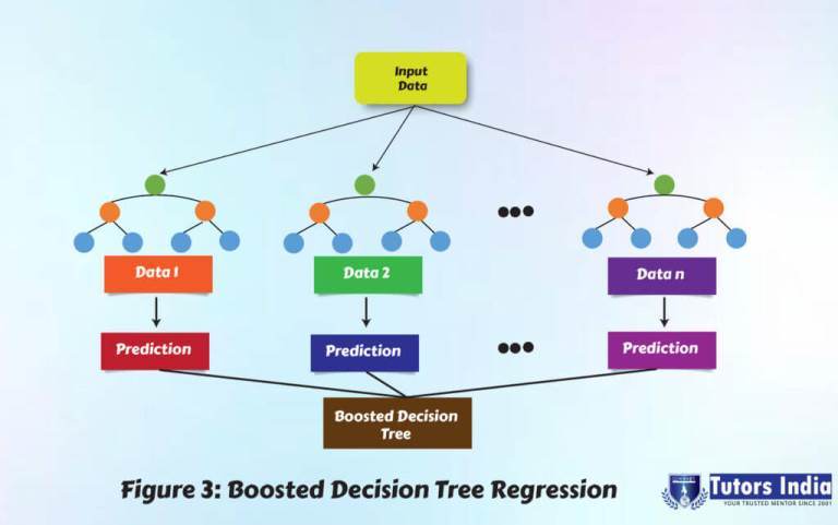
A BDTR is a classic method to create an ensemble of regression trees where each tree is dependent on the prior tree [36]. In ensemble learning methods, the second tree rectifies the errors of the primary tree, the errors of the primary and second trees are corrected by the third tree, and so on. Predictions are made using the entire set of trees used to create the forecast. The BDTR is particularly effective at dealing with tabular data. The advantages of BDTR are it robust to missing data and normally allocate feature significance scores.
BDTR usually outperforms DFR since it appears to be the method of choice in Kaggle competition, with somewhat better performance than DFR. Unlike DFR, BDTR is more prone to overfitting because the main purpose is to reduce bias and not variance. BDTR takes longer to build because there are more hyperparameters to optimize, and trees are generated sequentially [4].
Figure 1 shows the distribution of BDTR where the trees are generally shallow with three-parameter—number of trees, depth of trees, and learning rate [1].
Decision Forest Regression (DFR)
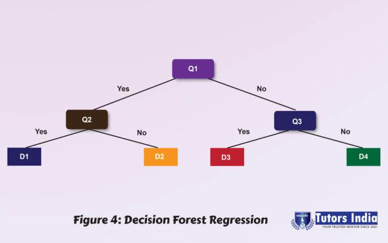
A DFR is a collective of randomly trained decision trees [5]. It works by constructing many decision trees at training time and produces a mean forecast (regression) or an individual tree model of classes (classification) as the end of the product. Each tree is assembled with a random subset of features and an irregular subset of data that allows the trees to deviate by appearing in different datasets. It has two parameters: the number of trees and the number of selected features at each node. DFR is good in generates uneven data sets with missing variables since it is generally robust to over fitting. It also has lower classification errors and better scores than decision trees, but it does not easily interpret the results. Another disadvantage is the important feature may not be vigorous to variety within the preparing dataset.
It has two parameters: the number of trees to be selected at each node and the number of features to be certain at each node. Because it is generally resistant to over fitting, DFR generates unequal data sets with missing variables. It also has lower classification error and f-scores than decision trees, but the findings are difficult to interpret. Another significant disadvantage is that the feature may not deal with the variability in the supplied dataset. The distribution of DFR is depicted in Figure 2 below[1].
Neural Network Regression (NNR)
NNR is made up of a series of linear operations interspersed with non-linear activation functions. The network’s settings are as follows: the foremost layer is the input layer, the former layer is the output layer, and some hidden layers are made up of the equal number of nodes to the number of classes [1].
the structure of a neural network (NN) model gives a brief description of the number of hidden layers, how the layers are connected, the number of nodes in each hidden layer, which activation function is used, and weights on the graph edges. Although NN is widely known for using deep learning and modelling complicated problems such as image recognition, it can be easily adapted to regression problems. If individuals employ adaptive weights and approximate the non-linear functions of their inputs, any statistical model can be classified as a NN. As a result, NNR is well suited to problems where a typical regression model cannot provide a solution. Figure 3 below shows the architecture modeling[1].
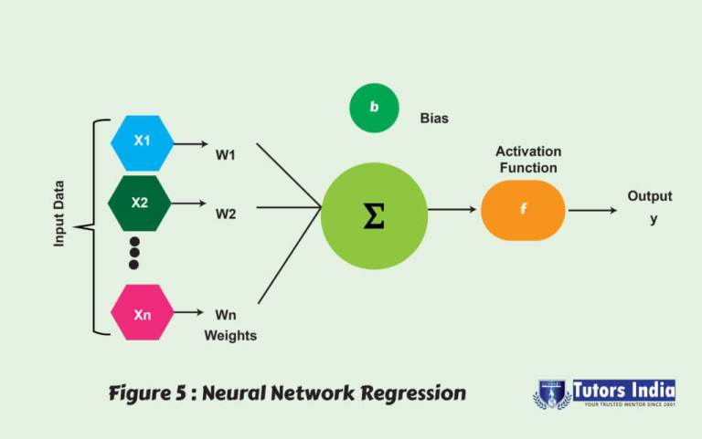
NNR is a sequence of linear operations scattered with various non-linear activation functions [41]. The network has these defaults; the major layer is the input layer, the last layer is the output layer, and the hidden layer consisting of several nodes equal to the number of classes [42]. A neural network (NN) is defined by its structure, including the number of hidden layers, each hidden layer’s number of nodes, how the layers are linked, which activation function is used, and the weights. NN’s are widely known for use in deep learning and modelling complex problems such as image recognition. They are easily adapted to regression problems. Thus, NNR is suited to situations where a more traditional regression model cannot fit a solution.
Bayesian Linear Regression (BLR)
Unlike linear regression, the Bayesian technique employs Bayesian inference [43]. To obtain parameter estimates, prior parameter information must be paired with a probability function. The forecast distribution utilizes probabilities by current belief about w given data to assess the likelihood of a value y given x for a specific w. (y, X). Finally, add up all of the potential w [43] values. BLR uses a natural mechanism to allow insufficient or incorrectly dispersed data to survive. The main benefit is that, unlike traditional regression, Bayesian processing allows you to recover the complete spectrum of inferential solutions rather than just a single estimate and a confidence interval.
To summarize, the choice of the proposed methods to implement the rainfall forecasting model is difficult for mimicking the rainfall process utilizing traditional model methods. The rainfall behaviour is affected by stochastic and natural resources such as the rise of temperatures when the air becomes warmer, more moisture evaporates from land and water to the atmosphere, and weather change causes shifts in air and ocean currents weather patterns.
Hire Tutors India experts to develop your algorithm and coding implementation for your Computer Science dissertation Services.
Performance evaluation metric for machine learning methods
The success of scoring (datasets) that has been by a trained model to replicating the true values of the output parameters listed as follows was measured using model performance evaluation.
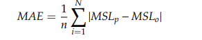
- MAE stands for Mean absolute error, reflecting the degree of absolute error between the actual and forecasted data.
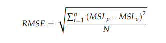
- RMSE stands for Root Mean Square Error is compared between the forecasted and the actual data.
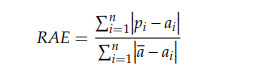
- RAE stands for Relative absolute error, is the relative absolute difference between the forecasted and the actual data.
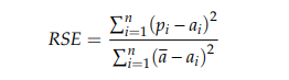
- RSE stands for Relative squared error [1], which similarly normalizes the entire squared error of the forecasted values.
- Coefficient of determination, R 2 [1] shows the forecasting methods’ performance where zero refers to the random model while one means there is a perfect fit.
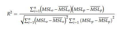
- In summary, predicting performance is better when R 2 is close to 1, but it differs for RMSE and MAE since the model’s performance is better when the value is close to 0.
Method 1: Forecasting rainfall using Autocorrelation Function (ACF)
It uses 4 various regression models: BDTR- Boosted Decision Tree Regression (), DFR- Decision Forest Regression , BLR- Bayesian Linear Regression, NNR- Neural Network Regression, and table 1 illustrate the best model to predict rainfall results based on ACF. Given that rainfall data is split into daily, weekly, 10-days, and monthly, each regression gives a different scenario. Since BDTR has the highest coefficient determination of R2, it is considered the best regression developed of ACF.
Table 1 Result for the best model in M1 using ACF [1]
| Scenario | Regression | Model | Coefficient of Determination |
| (a) Daily | |||
| Rt = Rt-1 | BDTR | Without tuning | 0.2458173 |
| With tuning | 0.5525075 | ||
| Rt + Rt -1 = Rt -2 | BDTR | Without tuning | 0.1383447 |
| With tuning | 0.8468193 | ||
| (b) Weekly | |||
| Rt = Rt-1 | BDTR | Without tuning | 0.0002462 |
| With tuning | 0.8400668 | ||
| Rt = Rt -49 | BDTR | Without tuning | 0.1179256 |
| With tuning | 0.8825647 | ||
| (c) 10 Days | |||
| Rt = Rt-1 | BDTR | Without tuning | 1.0041807 |
| With tuning | 0.8038288 | ||
| Rt = Rt -34 | BDTR | Without tuning | 0.1182632 |
| With tuning | 0.8949389 | ||
| (d) Monthly | |||
| Rt = Rt-1 | BDTR | Without tuning | 0.1163886 |
| With tuning | 0.9174191 | ||
| Rt = Rt -11 | BDTR | Without tuning | 0.0514856 |
| With tuning | 0.6941756 |
Based on these outcomes, it can be concluded that BDTR can accurately predict rainfall over various time horizons and that the model’s accuracy improved when more inputs were included.
Method 2: Forecasting rainfall using projected error
Table 2 summarizes the top three best models for different scenarios using different normalization and data partitioning metrics. In this context, different normalizations such as ZScore, LogNormal, and MinMax and data partitioning (80% and 90%) are investigated to obtain the optimal model with high accuracy.
Table 2: summarizes the top three best models for different scenarios using different normalization and data partitioning metrics. [1]
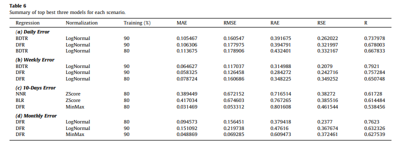
Except for the 10-day prediction, overall model performance indicates that normalizing using LogNormal produces good results for each category. The comparison between the BDTR and DFR models is the most acceptable result than NNR and BLR. The results show the best model for daily error prediction with R equal to 0.737978 is BDTR, and for weekly rainfall error prediction where R equal to 0.7921. While for monthly rainfall error prediction, DFR outperformed other models where R was equal to 0.7623. However, for 10-days rainfall error prediction, the NNR model with ZScore normalization outperformed other models in predicting the value of 10-days with an acceptable level of accuracy where R is equal to 0.61728. It can be concluded that an acceptable level of accuracy could be achieved by reducing the error in the dataset of the projected rainfall with the expected observable rainfall by using BDTR integrated with LogNormal and partitioning the data to 90% for training 10% for testing. Finally, Fig. 3 demonstrates the actual error and the predicted error. The figure shows how well the proposed model can resemble the observed and projected rainfall error during the testing phases. The red line demonstrates the predicted value from the proposed ML algorithm, while the blue line demonstrates the observed value of actual error. It can be seen that the projected model has an acceptable level of accuracy for all four different time horizons; however, the highest level of accuracy was obtained for the weekly error.
Conclusion
Method 1: The results presented that for M1, the result improves with cross-validation with BDTR and tuning its parameter. The more input included in the model, the more accurate the model can perform. BDTR is the best ACF regression because it has the highest coefficient of determination, R2 (daily: 0.5525075, 0.8468193, 0.9739693; weekly: 0.8400668, 0.8825647, 0.989461; 10 days: 0.8038288, 0.8949389, 0.9607741, 0.9894429; and monthly: 0.9174191, 0.6941756, 0.9939951, 0.9998085) meaning the better rainfall prediction for the future.
Method 1 is the best prediction for the rainfall, mimicking the actual values with the highest coefficient closer to 1. The dependencies on ACF show that rainfall has almost a similar pattern every year from November to January, and this shows a correlation between the predicting input and output. The current study’s findings showed that standalone machine-learning algorithms can predict rainfall with an acceptable level of accuracy; however, more accurate rainfall prediction might be achieved by proposing hybrid machine learning algorithms and with the inclusion of different climate change scenarios.
Tutorsindia assists numerous Uk Reputed universities students and offers outstanding Machine Learning dissertation and Assignment help Also offers full dissertation writing service across all the subjects. No doubt, we have subject-Matter Expertise to help you in writing the complete thesis. Get Your PhD Research from your Academic Tutor with Unlimited Support!
References
- Ridwan, W. M., Sapitang, M., Aziz, A., Kushiar, K. F., Ahmed, A. N., & El-Shafie, A. (2021). Rainfall forecasting model using machine learning methods: Case study Terengganu, Malaysia. Ain Shams Engineering Journal, 12(2), 1651-1663.
- Ghumman, A. R., Ghazaw, Y. M., Sohail, A. R., & Watanabe, K. (2011). Runoff forecasting by artificial neural network and conventional model. Alexandria Engineering Journal, 50(4), 345-350.
- Wahab, N. A., Kamarudin, M. K. A., Toriman, M. E., Juahir, H., Gasim, M. B., Rizman, Z. I., … & Ata, F. M. (2018). Climate changes impacts towards sedimentation rate at Terengganu River, Terengganu, Malaysia. Journal of Fundamental and Applied Sciences, 10(1S), 33-51.
- Nakagawa, S., & Freckleton, R. P. (2008). Missing inaction: the dangers of ignoring missing data. Trends in ecology & evolution, 23(11), 592-596.
- Criminisi, A., Shotton, J., & Konukoglu, E. (2012). Decision forests: A unified framework for classification, regression, density estimation, manifold learning and semi-supervised learning. Foundations and trends® in computer graphics and vision, 7(2–3), 81-227.
 Previous Post
 Next Post